Face Detection with Tensorflow Rust
Using MTCNN with Rust and Tensorflowrust 2019-03-28
One of the promises of machine learning is to be able to use it for object recognition in photos. This includes being able to pick out features such as animals, buildings and even faces.
This article will step you through using some existing models to accomplish face detection using rust and tensorflow. For the impatient among you, you can find the source code here: https://github.com/cetra3/mtcnn
We will be using a pre-trained model called mtcnn for face detection (Note: training a new model is not something we'll be concerned with in this article).
The Challenge
We want to read the photo, have the faces detected, and then return an image with the bounding boxes drawn in.
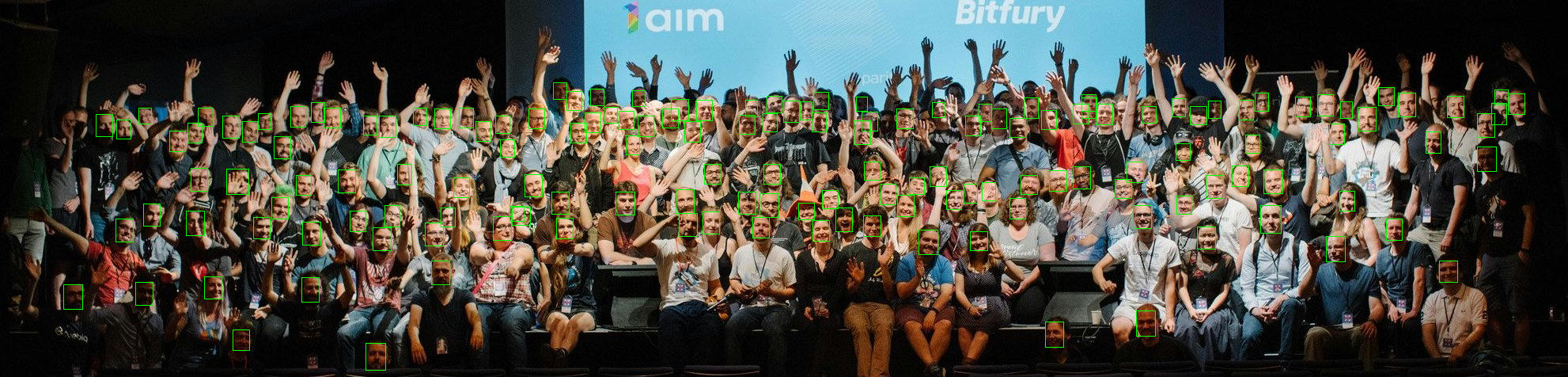
In other words, we want to convert this (Image used with permission of RustFest, taken by Fiona Castiñeira):

Into this:
Tensorflow and MTCNN
The original MTCNN model was written using Caffe, but luckily there is a number of tensorflow python implementations for mtcnn. I'm going to pick the following as it is a straight conversion into a single graph model file.
Firstly we want to add tensorflow rust as a dependency. Here's a Cargo.toml to start:
[package]
name = "mtcnn"
version = "0.1.0"
edition = "2018"

[dependencies]
tensorflow = "0.12.0"
What we're going to do is load a Graph which is the pre-trained MTCNN, and run a session. The gist is that a Graph is the model used for computation, and a Session is one run of the Graph. A lot more information about these concepts can be found here. I like to think of the Graph as an artificial brain in a vat, just to get some great imagery when you start plugging in inputs and outputs.
So let's start by grabbing the existing mtcnn.pb model and trying to load it up. Tensorflow graphs are serialised out in protobuf format and can be loaded in using Graph::import_graph_def.
use std::error::Error;

use tensorflow::Graph;
use tensorflow::ImportGraphDefOptions;

fn main() -> Result<(), Box<dyn Error>> {

    //First, we load up the graph as a byte array
    let model = include_bytes!("mtcnn.pb");

    //Then we create a tensorflow graph from the model
    let mut graph = Graph::new();
    graph.import_graph_def(&*model, &ImportGraphDefOptions::new())?

    Ok(())
}
Running cargo run we should see no errors:
$ cargo run
   Compiling mtcnn v0.1.0 (~/mtcnn)
    Finished dev [unoptimized + debuginfo] target(s) in 0.89s
     Running `target/debug/mtcnn`
Great! Looks like we can load the graph!
StructOpt and the Command Line
We're going to want to test out image generation, so let's use structopt to take two arguments: input and output.
If you haven't used structopt before: structopt is like combining clap with serde. The input argument will be the path of an image file. The output will be where we save the output image.
So our struct looks like this:
use std::path::PathBuf;
use structopt::StructOpt

#[derive(StructOpt)]
struct Opt {
    #[structopt(parse(from_os_str))]
    input: PathBuf,

    #[structopt(parse(from_os_str))]
    output: PathBuf
}
The parse(from_os_str) attribute will convert a string argument directly into a PathBuf to save us some boiler plate
We can then use this to get a struct with our command line arguments
fn main() -> Result<(), Box<dyn Error>> {

    let opt = Opt::from_args();
    ....
}
Loading Image Data
We need to provide the tensorflow graph with our image data. So how do we do that? We use a Tensor! Tensors represent data within our graph, it sort of reminds me of sending vertices to a GPU. You have a big slice of data, and send it in a format that tensorflow is expecting.
The input tensor in this graph is an array of floats, with dimensions: height x width x 3 (for 3 colour channels).
Let's use the image crate to load the image:
let input_image = image::open(&opt.input)?;Next we want to convert this image into its raw pixels by using the GenericImage::pixels function and send that to our graph. All multi-dimensional Tensor arrays are flat, and stored in row major order. The model uses BGR instead of the traditional RGB for colours, so we'll need to reverse the pixel values when we iterate through.
Putting it all together:
let mut flattened: Vec<f32> = Vec::new();

for (_x, _y, rgb) in input_image.pixels() {
    flattened.push(rgb[2] as f32);
    flattened.push(rgb[1] as f32);
    flattened.push(rgb[0] as f32);
}
This simply iterates through the pixels, adding them to a flattened Vec.
We can then load this into a tensor, specifying the image height and width as arguments:
let input = Tensor::new(&[input_image.height() as u64, input_image.width() as u64, 3])
    .with_values(&flattened)?
Great! we have loaded our image into a format that the graph understands. Let's run a session!
Creating a tensorflow session
Ok, we have a graph, the input image, but now we need a session for the graph. We'll just use the defaults for this:
let session = Session::new(&SessionOptions::new(), &graph)?;Running a session
Before we run a session, we have a few other inputs the mtcnn model is expecting. We're gonna use the same defaults the mtcnn library for these values:
let min_size = Tensor::new(&[]).with_values(&[40f32])?;
let thresholds = Tensor::new(&[3]).with_values(&[0.6f32, 0.7f32, 0.7f32])?;
let factor = Tensor::new(&[]).with_values(&[0.709f32])?;
The graph can define multiple inputs/outputs that are required before running and it depends on the specific neural net as to what these are. For MTCNN, these are all described in the original implementation. Probably the most important one is the min_size which describes the minimum size to find faces.
Now we build the session arguments for the inputs:
let mut args = SessionRunArgs::new();

//Load our parameters for the model
args.add_feed(&graph.operation_by_name_required("min_size")?, 0, &min_size);
args.add_feed(&graph.operation_by_name_required("thresholds")?, 0, &thresholds);
args.add_feed(&graph.operation_by_name_required("factor")?, 0, &factor);

//Load our input image
args.add_feed(&graph.operation_by_name_required("input")?, 0, &input);
Ok, what about outputs? There are two that we are going to request when the session is finished: bounding boxes and probabilities:
let bbox = args.request_fetch(&graph.operation_by_name_required("box")?, 0);
let prob = args.request_fetch(&graph.operation_by_name_required("prob")?, 0);
Ok cool, we have our inputs, and our outputs, let's run it!
session.run(&mut args)?;The BBox struct
The model outputs the following values:
- Bounding box of the faces
- Landmarks of the faces
- Probability that it's a face from
0to1
In order to make it a bit more easy to work with, we'll define a bounding box struct which encodes those values back in a more easy to read fashion:
#[derive(Copy, Clone, Debug)]
pub struct BBox {
    pub x1: f32,
    pub y1: f32,
    pub x2: f32,
    pub y2: f32,
    pub prob: f32,
}
We'll omit landmarks for simplicity, but can always add them back if we need. Our job is to convert the arrays we get back from the tensorflow session into this struct so it's more meaningful.
Saving the Output
Right, now let's grab back the outputs. Just like inputs, outputs are Tensors too:
let bbox_res: Tensor<f32> = args.fetch(bbox)?;
let prob_res: Tensor<f32> = args.fetch(prob)?;
What is the shape of bbox? Well, it's a multi-dimensional flattened array that includes 4 floats per bounding box representing the bounding box extents. The prob is an array with a single float value per face: the probability from 0 to 1. So we should expect the bbox_res length to be the number of faces x 4, and prob_res to be equal to the number of faces.
Let's do some basic iteration and store our results into a Vec:
//Let's store the results as a Vec<BBox>
let mut bboxes = Vec::new();

let mut i = 0;
let mut j = 0;

//While we have responses, iterate through
while i < bbox_res.len() {

    //Add in the 4 floats from the `bbox_res` array.
    //Notice the y1, x1, etc.. is ordered differently to our struct definition.
    bboxes.push(BBox {
        y1: bbox_res[i],
        x1: bbox_res[i + 1],
        y2: bbox_res[i + 2],
        x2: bbox_res[i + 3],
        prob: prob_res[j], // Add in the facial probability
    });

    //Step `i` ahead by 4.
    i += 4;
    //Step `i` ahead by 1.
    j += 1;
}
Combinators
Alternatively, we could use combinators to replace the one above.
let bboxes: Vec<_> = bbox_res
    .chunks_exact(4) // Split into chunks of 4
    .zip(prob_res.iter()) // Combine it with prob_res
    .map(|(bbox, &prob)| BBox {
        y1: bbox[0],
        x1: bbox[1],
        y2: bbox[2],
        x2: bbox[3],
        prob,
    })
    .collect();
Printing out the bounding boxes
Ok, we haven't encoded the bounding boxes into an image, yet. but let's debug to make sure we're getting back something:
println!("BBox Length: {}, Bboxes:{:#?}", bboxes.len(), bboxes);Running this, what do we get back:
BBox Length: 120, BBoxes:[
    BBox {
        x1: 471.4591,
        y1: 287.59888,
        x2: 495.3053,
        y2: 317.25327,
        prob: 0.9999908
    },
    ....
Whoa! 120 faces! Awesome!
Drawing the Bounding Boxes
Great, we have some bounding boxes. Let's draw them on the image, and save the output into a file.
To draw bounding boxes, we can use the imageproc library to draw simple borders around the bounding boxes.
Firstly, we'll make the line colour constant green outside of our main() function:
const LINE_COLOUR: Rgba<u8> = Rgba {
        data: [0, 255, 0, 0],
};
Now stepping back into it. We are feeding in the input image read only, so let's use the first image to draw onto:
let mut output_image = input_image;Then we iterate through our bounding boxes:
for bbox in bboxes {
    //Drawing Happens Here!
}
Next, we use the draw_hollow_rect_mut function. This will take a mutable image reference, and draw a hollow rectangle (outline) specified by the input Rect, overwriting any existing pixels.
The Rect takes an x and y coordinate with the at function, and then a width and height with the of_size function. We use a bit of geometry to convert our bounding box to this format:
let rect = Rect::at(bbox.x1 as i32, bbox.y1 as i32)
    .of_size((bbox.x2 - bbox.x1) as u32, (bbox.y2 - bbox.y1) as u32);
Then draw the rect:
draw_hollow_rect_mut(&mut output_image, rect, LINE_COLOUR);Once the for loop is done, we save it in the output file:
output_image.save(&opt.output)?;And we're done. Let's run it!
$ cargo run rustfest.jpg output.jpg
   Compiling mtcnn v0.1.0 (~/mtcnn)
    Finished dev [unoptimized + debuginfo] target(s) in 5.12s
     Running `target/debug/mtcnn rustfest.jpg output.jpg`
2019-03-28 16:15:48.194933: I tensorflow/core/platform/cpu_feature_guard.cc:141] Your CPU supports instructions that this TensorFlow binary was not compiled to use: SSE4.2 AVX AVX2 FMA
BBox Length: 154, BBoxes:[
    BBox {
        x1: 951.46875,
        y1: 274.00577,
        x2: 973.68304,
        y2: 301.93915,
        prob: 0.9999999
    },
....
Looks good, no errors!
Wrapping up
Let's step through what we've done in this little application:
- Loaded a pre-trained tensorflow graph
- Parse the command line arguments
- Read in image data
- Extracted faces by running a tensorflow session
- Saved the results of that session back to the image
- Wrote out the file
If you got stuck at any point, have a look at the repository here: https://github.com/cetra3/mtcnn
Hopefully this gives you a good introduction to using tensorflow in rust